If you reached here by chance, just be sure of reading the first part of the post first, in which we explain why a Drought Monitor is necessary. In this second part, you can find a longer description of the technical aspects of the development of this prototype.

Technicalities

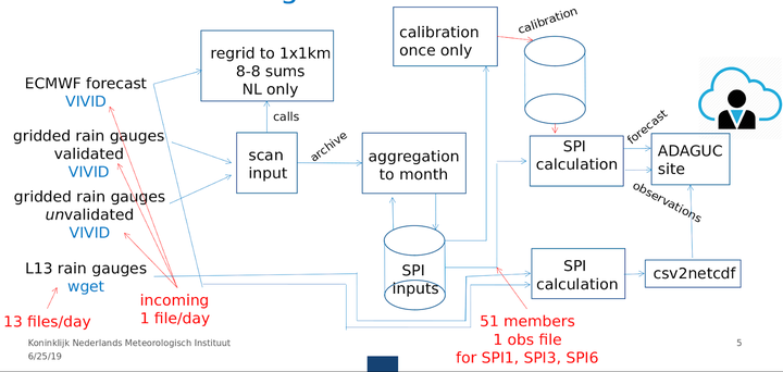
This section does not intend to be an exhaustive description of the processing required to develop the prototype, but to provide a high level description. The image below shows the workflow that we implemented:

Processing rainfall data

We obtained daily gridded precipitation datasets from the KNMI repositories for the period 1951-2019 (up to 11/06/19) at 1km resolution, and downloaded the 15-day forecast from ECMWF (from 12/06/19 onwards). All these files are available in NetCDF format. The daily gridded precipitation files are aggregated to a 1, 3, or 6 months resolution, which means that for each day in the time-series the resulting file NetCDF file will contain the accumulated precipitation over the previous 30, 90, or 180 days. The 15-day forecast files from ECMWF are regridded to 1km resolution and they are temporally organized so the time dimension matches the one of the precipitation datasets. All these files are stored in the “SPI inputs” database.

Calculating the standard precipitation index (SPI)

The computation of the SPI is based on an adaptation of a method developed by the USA NIDIS (National Integrated Drought Information System), available in this link. This organization provides Python implementations of several climate index algorithms along the SPI (SPEI, PMDI). The SPI index is computed by fitting a Gamma distribution to the gridded dataset of precipitation accumulation within the calibration period. The WMO recommends a calibration period of, at least, 30 years. In our case, we have available 68 years of precipitation data (1951-2019), thus, we define our calibration period as 1951-2010 and we will used the fitted distributions to forecast for the period 2011-2019.

The original NIDIS SPI routine does not keep the coefficients of the fitted Gamma distributions, it just provides the value of the SPI index. Hence, we modified the original code to keep these parameters (alpha, beta, probability of no rain) and use them again during the forecasting stage. The modified SPI routine will take the time-series accumulation of precipitation for each of the grid cells in the country, and will fit a Gamma distribution to this array, keeping the coefficients. After this procedure we create a NetCDF file containing the predicted SPI within the calibration period and another one with the coefficients of the Gamma distribution that are used in forecasting.

The forecasting implies two stages (and a tongue twister): Using the Gamma coefficients obtained during the first stage we reconstruct the distribution in a per-pixel basis and we forecast the daily SPI for the period 2011-2019. We apply the same forecasting procedure to the 15-day forecast from ECMWF, thus obtaining the expected SPI within the next 15 days. This procedure creates multiple daily NetCDF files containing the SPI values that are ready to be integrated in a web application.

Operationalisation

We selected ADAGUC server to host and make the data available as a webservice that later on can be incorporated in any website. We chose this platform because it allows the continuous expansion of the dataset as new observations come in, it can render maps and time series directly from NetCDF files, and we can query map images following the WMS standard of OGC. Regarding the frontend, we create a web application written in Javascript based on React-Redux libraries, and we visualize maps using the new ADAGUC geographic mapping component. The code contributed by all the participants was hosted in Gitlab, which allowed version control and continuous integration and deployment (CI/CD). This means that no human action is needed to trigger and complete the deployment pipeline. We configured CI/CD to deploy the front end to an AWS S3 bucket and ADAGUC server to an AWS EC2 node. Upon deployment, the data on the underlying AWS-EFS file system is synced with data uploaded to S3 staging buckets.